Lab 8: Centripetal Acceleration vs. Angular Frequency 3/25/15

Physics Lab #8 started on 3/25/15
Centripetal Acceleration vs. Angular Frequency
Annemarie Branks
Professor Wolf

Objective: Determine the relationship between centripetal acceleration and angular speed.

Procedure:
     1.  This was a class demonstration because there was only one apparatus, which was a voltage box connected to a wheel which spun our heavy rotating disk. The voltage box allowed us to have a constant angular velocity for the disk. We turned on the the box at 4.4 volts and used our photogate and LoggerPro to determine the period of one rotation which we used to determine angular velocity. We then took data  from the accelerometer to determine its centripetal acceleration.

     2.  Repeat the process for increasing angular speed. We repeated this process for 6.4, 8.6, 9.6, and 10.8 volts. 
     3.  Since centripetal acceleration = r*ѡ^2, make a graph of ѡ^2 by centripetal acceleration. The graph's slope should give you the radius of the rotating disk.

     4.  Compare the slope of your graph to the actual radius of the rotating disk. Our actual radius was 13.8 cm which is equal to 0.138 m. This is very accurate to the answer we got from the graph, so the experiment was a success with showing the relationship between the centripetal acceleration and angular speed.

Lab 7: Trajectories 3/23/15

Physics Lab #7 started on 3/23/15
Trajectories
Annemarie Branks
Professor Wolf

Objective: Predict where a ball, flying off of a track, will hit a board angled below the track.

Procedure:
     1.  Securely set up the apparatus using a liberal amount of masking tape to keep the track static. Mark a part of the track where you will launch the ball from for each trial.

     2.  Using a weight tied to a string, mark the floor with tape to indicate where the ball leaves the track. You will use this marking to measure how high the ball is from the ground when it launches and how far it launches in the x-direction.
     3.  Tape carbon paper to the floor. Release the ball from the same place five times and measure how far in the x-direction the ball launched. Our average horizontal distance is 50.5 cm +/- 0.3cm. 

     4.  Knowing the distance in the x-direction, and having measured the distance in the y-direction (94.2 +/- 0.1 cm) we can determine how fast the ball is leaving the track. This is how we solved for V0x:

     5.  Set up a wooden board directly below the track at angle. We are going to solve for the distance the ball traveled in relation to the board. We need to know the board's angle, the height from which the ball launches, and the ball's initial velocity which we found from step 4. Here are the calculations for our experiment:

     6.  Cover the board with carbon paper. Then launch the ball 5 times and measure the distance from the track. Make sure neither the board nor the track moves at all.

     7.  Measure how far on the board your ball made its marks and see if your actual data matches up with your calculated data from step 5. Our experiment gave us an average distance of 48.02 +/- 0.52 cm. Your numbers may not match up due to uncertainties in measurements. Calculate the range on uncertainty for d. 
Our equation is d = (2*V0x^2sinα)/(g(cosα)^2) which, if you trace back your steps in calculating d, you will find simplifies to (sinα*x^2)/(ycos^2α). This can also be written as (x^2/y)tanαsecα. We are going to use the second equation so we can use product rule when it comes time to derive. 

d = (x^2/y)tanαsecα

dd = |∂d/∂y|dy + |∂d/∂x|dx + |∂d/∂α|dα

dd = |(-x^2/y^2)tanαsecα(0.1)| + |(2x/y)tanαsecα(0.3)| + |(x^2/y)(secαtan^2α+sec^3α)(0.035)|

dd = 0.133+0.915+5.267 = 6.315

With our uncertainties in measurements, the distance the ball traveled in reference to the board should be 47.47 +/- 6.315 cm. This range is fairly large which is not ideal but it matches up well with the actual average distance of 48.02 +/- 0.52 cm.

Lab 6: Modeling Friction Forces 3/16/15

Physics Lab #6 started on 3/16/15
Modeling Friction Forces
Annemarie Branks
Professor Wolf

Part 1:
Objective: Determine the coefficient of static friction between two surfaces by graphing the normal forces and frictional forces for an increasing number of masses. 

Procedure:
     1.  With your block on the table, and the string tied to the Styrofoam cup hanging over the edge via "Atwood" pulley, begin slowly filling your Styrofoam cup with water until you just barely see the block begin to move.

     2. Measure the mass of the cup and the water on a scale. In kilograms, multiply the mass by the force of gravity. This number will be equivalent to the max static friction force of the block. 

     3. Repeat steps 1 and 2 with an additional block for a total of four trials. You will also need to weigh the mass of the blocks  in each trial to find their Normal Forces.

     4. From this information we can create a Max Static Friction Force by Normal Force graph and find a best of fit equation. The slope of the graph will give us the coefficient of static friction for the block against the table. The line on the graph must intercept the origin.

Our μ for static friction is 0.3267.

    

Part 2:

Objective: Determine the coefficient of kinetic friction between two surfaces by graphing the normal forces and frictional forces for an increasing number of masses. 

Procedure: 

     1.  Tie a force sensor to your first wooden block that will remain in contact with the table through out the entire experiment. After you've set up the force sensor with LoggerPro and zeroed it, you can begin collecting data by pulling on the force sensor horizontal to the table at a constant speed.

     2.  Obtain the average force exerted on the block from LoggerPro.

     3.  Record your mass of the block so you can find its Normal Force.

     4.  Repeat steps 2 and 3 for a total of four trials, with each trial having an additional mass.

     5.  Just like in Part One, make a graph in excel to find the coefficient of friction, but only this time it will be for kinetic friction. It would make sense that the coefficient for kinetic friction is smaller than the coefficient for static friction.

Our μ for kinetic friction is 0.2675.

Part 3:

Objective: Find the angle at which the block begins to slip to determine the coefficient of static friction between the block and the surface.

Procedure:

     1.  Place your block on a track that you can move up and down. Have a lab partner hold down one end of the track so that it does not move and affect the results. 

     2.  Slowly raise one end of the track and watch for when the block begins to slide down. At the moment, record the angle of the track. Our angle was 13.5° +/- 0.1°.

     3.  You may want to draw out a diagram displaying all the forces acting upon the block. Solve for μ for kinetic friction. In our case it was 0.2401.

Part 4:

Objective: Determine the coefficient of kinetic friction for an object sliding down a slope.

Procedure:

     1.  Set up a track to rest on a stand at an angle large enough to cause the block resting on it to move. Record that angle.

     2.  Keeping the track at that angle, set up the motion detector at the top end of the track so you can determine the block's acceleration.

     3.  With the determined values for the block's acceleration, the track's incline, and the mass of the block, we can solve for μ for kinetic friction. For our experiment, LoggerPro gave us an acceleration of 1.079 m/s^2, the track was at an incline of 24.3°, and the mass of the block was 0.1264 kg. 

From the sum of forces in the y direction, we found that the Normal = 1.13N. Using Normal*μ to replace Frictional force, we solved for μ and got a value of 0.33.

Part 5:

Objective: With our new found coefficient for kinetic friction from Part 4, calculate an expression for what the system's acceleration should be if the track were laid horizontally.

Procedure:

     1.  Create a system where the block is still on the track and will accelerate due to a hanging mass. You will use LoggerPro to find the actual acceleration of the system so you can compare it to the your calculated acceleration.

     2.  Before you start the physical experiment, find your calculated acceleration. Here is our calculation for acceleration.

     3.  We can now collect our data via LoggerPro when we let go of the hanging mass and find acceleration. Our acceleration was 0.6911 m/s^2. This means our percentage difference was 40.15% which seems large but Professor Wolf said the percentage difference should be off by about 50%. This could be because of inconsistency in our track and string tension as well as not considering the pulley as a part of the system.

Lab 5: Modeling the fall of an object with air resistance 3/11/15

Physics Lab #5 started on 3/11/15
Modeling the fall of an object with air resistance
Annemarie Branks
Professor Wolf

Objective: Determine the relationship between air resistance and speed. Model the fall of an object including air resistance.

Procedure:
     1. We want to be able to drop an object that would be subjective to air resistance but still be able to drop straight down without moving left and right like a feather would. Coffee filters worked out great for this experiment. We need to find the object's terminal velocity so we have to drop it from a high enough location so that can happen.

     2.  For each trial we dropped an increasing number of coffee filters from a high balcony while recording a video of the experiment on LoggerPro. The person who dropped the coffee filters also held a meter stick so that we could tell LoggerPro how long a meter is in the image. We stopped the experiment after dropping five coffee filters together.

     3.  In LoggerPro we made a position graph for each trial and highlighted the section with a relatively straight slope and made a linear fit. This slope is the experimental velocity for a given amount of coffee filters dropped. Below is an example of the experimental velocity for four coffee filters dropped.

     4. From the overall look of the position graph we are assuming that the Force of air resistance will equal to velocity to some power times some constant or F=kv^n. We have decided that the origin is where we first dropped the coffee filter and that the direction it is falling in is the positive direction. So if we did a Newton's Second Law equation, it would look like:

mg-kv^n=ma

a=g-(k/m)*v^n

     5.  The next step is setting up a spreadsheet so we can decide what the values of k and n are. K and n describe the object's shape. We listed the Velocity and Force Resistance for each trial. We already know the velocity from the slope we got in LoggerPro and the Force Resistance at terminal velocity is simply the mass times the acceleration of gravity. We found from weighing 50 coffee filters that one coffee filter is 0.000926 +/- 0.000002 kg. From there we made a graph, did a power trend line, and obtained the following results:

From the given equation we now have values for k and n. k=0.0108 and n=2.0596. The values of k and n have an uncertainty of 5%.

     6.  Now that we have an acceleration for for the coffee filters, we can plug in our equation into an Excel spreadsheet to see if our terminal velocity matches the one that we got from LoggerPro. Here are the visible equations we plugged in to show how we got our values:

     7.  In the cell for mass (I4) we can change how many times the mass is multiplied by to indicate the number of coffee filters we want to find the terminal velocity for.

For one coffee filter we have found from Excel that the terminal velocity is 0.9189678 m/s.

For two coffee filters we have found from Excel that the terminal velocity is 1.286648 m/s.

For three coffee filters we have found from Excel that the terminal velocity is 1.5665979 m/s.

For four coffee filters we have found from Excel that the terminal velocity is 1.8014375 m/s.

For five coffee filters we have found from Excel that the terminal velocity is 2.0075762 m/s.

     8.  We can now determine how close the terminal velocities we found were to the terminal velocities found in LoggerPro. The first trial with just one coffee filter, had terminal velocities that have a percentage difference of 5.10%. The second trial with two coffee filters, had terminal velocities that have a percentage difference of 4.48%. The third trial with three coffee filters, had terminal velocities that have a percentage difference of 5.40%. The fourth trial with four coffee filters, had terminal velocities that have a percentage difference of 4.10%. 

The fifth trial with five coffee filters, had terminal velocities that have a percentage difference of 2.66%.

Conclusion:

Considering that k and n had a 5% error, our velocities turned out to be similar; however, 5% is still a significant difference in values. If we wanted to lower the percent difference of our values we would need more money to buy a better laptop, camera, and programs like LoggerPro and Excel, as well as more time to do the experiment. 

Lab 4: Propagated Uncertainty in Measurements 3/4/15

Physics Lab #4: Started on 3/4/15
Propagated Uncertainty in Measurements
Annemarie Branks
Professor Wolf

Objective: Determine the amount of uncertainty in calculated measurements. The first part of the lab will determine the uncertainty for density (ρ) and the second part will determine the uncertainty for the mass of a hanging object.

PART 1:

Procedure: 
     1.  With three metal cylinders, determine the measurements that will allow you to calculate their densities. The height and the diameter were determined by vernier calipers which have an uncertainty of ±0.01 cm. We then calculated for volume. V=π(d/2)^2*h

     2.  Measure the mass with a scale. Our scale had an uncertainty of ±0.1 g.

We can now calculate the density for each mass.

#1:  ρ = 4.28 g/cm^3

#2:  ρ = 2.89 g/cm^3

#3:  ρ = 9.22 g/cm^3

     3.  Before we try to determine what kind of metals these are based on their densities, we must acknowledge that they may be error due to the inaccuracy in measuring. To find the uncertainty in density we must do calculations for each metal.

ρ = m/v = (4/π)*m/(d^2*h)

dρ = |∂ρ/∂m|dm + |∂ρ/∂d|dd + |∂ρ/∂h|dh

dρ = |4/(πd^2*h)|dm + |-8m/(πd^3*h)|dm + |-4m/(πd^2*h^2)|dh

     4.  With the equation above, we can determine the uncertainty of the metals' densities.

For #1: dρ = 0.00688 + 0.0446 + 0.00852 = ±0.0600 g/cm^3 (with three sig figs)

For #2: dρ = 0.0158 + 0.0459 + 0.00569 = ±0.06739 g/cm^3

For #3: dρ = 0.0163 + 0.148 + 0.0184 = ±0.1827 g/cm^3

     5.  Each metal now has a range of values for its density. If you were to compare the values to accepted values you might be able to guess what kind of metal they each are.

#1:  ρ = 4.28 ±0.0600 g/cm^3

#2:  ρ = 2.89 ±0.06739 g/cm^3

#3:  ρ = 9.22 ±0.1827 g/cm^3

Results:

     The first metal had a density that didn't exactly match up with anything but was close to Selenium, Titanium, and Yttrium.

     The second metal, which we had guessed to be aluminum, does not include the density of aluminum in its range but came relatively close at 2.7 g/cm^3. Other metals that also came close are Boron, Carbon, Scandium, Silicon, and Strontium.

     The third metal, which we had guessed to be copper, yet again did not include the accepted density within its range, but came close at 8.92 g/cm^3. Erbium was the only element whose accepted density fell within our range but it was most likely not erbium because erbium doesn't have that bronze-like color. Other metals that came close to our range included Cobalt and Nickle.

Errors:

Possibilities for not being able to identify the substance

• The metals could have been alloys and I only compared their densities to pure substances.
• The metals could have slightly oxidized thus increasing their masses which would have increased the density. 
• The metal cylinders may have not been made properly, meaning they could have tiny air pockets inside them that would decrease their density.

Link to the site I used that lists densities: http://periodictable.com/Properties/A/Density.al.html

PART 2:

Procedure:
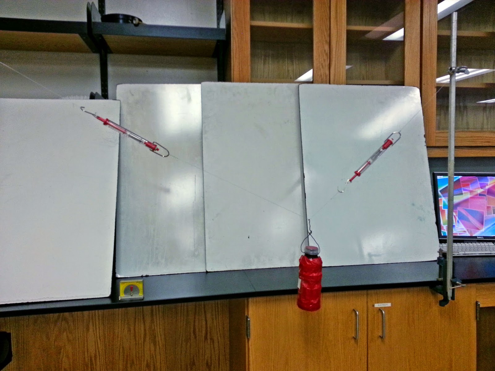
     1.  Professor Wolf set up hanging masses with spring scales. To begin determining the mass of the object we must record the forces pulling on the object. 

The top picture were going to call unknown mass 1 and the bottom unknown mass 2. From the spring scales we read the tension in the string. We also used a device that allowed us to find the degree of the string above the horizontal. The springs had an error of +/- 0.5 Newtons and the degree measuring device had an error of +/- 2° which is +/- 0.034906585 radians. Below is a picture of the device.

Here are the measurements we got for two of the hanging masses:

 

     2.  Determine the masses by calculating the forces in the y direction. We don't really care about what is happening in the x direction but it will let u know if your measurements are too inaccurate.

For unknown mass 1:

4.8*sin(26°)+6.4*sin(46°)=m1g

m1=6.708/g

m1=0.684 kg

For unknown mass 2:

10.7*sin(48°)+7.2*sin(11°)=m2g

m2=9.325/g

m2=0.951 kg

     3.  Just as we did for Part 1, we have to determine the rage of uncertainty for each mass. 

m = (F1*sinθ1 + F2*sinθ2)/g

dm = |∂m/∂F1|dF1 + |∂m/∂F2|dF2 + |∂m/∂θ1|dθ1 + |∂m/∂θ2|dθ2

dm = [|sinθ1|dF1 + |sinθ2|dF2 + |F1cosθ1|dθ1 + |F2cosθ2|dθ2]/g

For unknown mass 1:

dm = [|sin26°|0.5 + |sin46°|0.5 + |4.8*cos26°|0.0349 + |6.4cos46°|0.0349]/g

dm = 0.0901712891 kg

For unknown mass 2: 

 dm = [|sin48°|0.5 + |sin11°|0.5 + |10.7*cos48°|0.0349 + |7.2cos11°|0.0349]/g

dm = 0.098216 kg

Result:

For unknown mass 1: m = 0.684 +/- 0.0902 kg

For unknown mass 2: m = 0.951 +/- 0.0982 kg

What we learned:

This experiment showed that though we take our measurements as best as we can, there is a certain amount that we are unsure of in each measurement. We can calculate how uncertain we are and then find a range of values that should contain the actual value we are looking for.